Definite Integrals and Improper Integrals
Definite Integrals
I. Concept of Definite Integral
1. Definition
\[\begin{align} &\text{Definition: Let } f(x) \text{ be a function defined and bounded on the interval } [a,b].\\ &(1) \text{ Partition: Divide } [a,b] \text{ into } n \text{ subintervals } [x_{i-1},x_{i}].\\ &(2) \text{ Summation: Choose a point } \xi_{i} \text{ in } [x_{i-1},x_{i}], \text{ form the sum } \sum_{i=1}^{n}{f(\xi_{i})\Delta x_i}, \text{ where } \lambda=\max\{\Delta x_{1},\Delta x_{2},\dots,\Delta x_{n}\}.\\ &(3) \text{ Limit: If } \lim_{\lambda \rightarrow 0}{\sum_{i=1}^{n}f(\xi_{i})\Delta x_i} \text{ exists, and the limit value does not depend on the method of}\\ &\text{partitioning } [a,b] \text{ or the choice of points } \xi_{i}, \text{ then } f(x) \text{ is said to be integrable on } [a,b], \text{ and denoted as:}\\ &\int^{b}_{a}{f(x)dx}=\lim_{\lambda \rightarrow 0}{\sum_{i=1}^{n}f(\xi_i)\Delta x_{i}}\\ &\\ &\text{Notes:}\\ &(1) \lambda \rightarrow 0 \Rightarrow n \rightarrow \infty, \text{ but } n \rightarrow \infty \text{ does not necessarily imply } \lambda \rightarrow 0.\\ &(2) \text{ A definite integral represents a specific value, which depends on the interval } [a,b] \text{ but is independent of the variable of integration } x.\\ &\int_{a}^{b}{f(x)dx}=\int_{a}^{b}{f(t)dt}\\ &(3) \text{ If the integral } \int_{0}^{1}{f(x)dx} \text{ exists, divide } [0,1] \text{ into } n \text{ equal parts. Then } \Delta{x_{i}}=\frac{1}{n}. \text{ Choosing } \xi_{i}=\frac{i}{n}, \text{ we get:}\\ &\int_{0}^{1}f(x)dx=\lim_{\lambda \rightarrow 0}{\sum_{i=1}^{n}{f(\xi_{i})\Delta x_{i}}}=\lim_{n\rightarrow \infty}\sum_{i=1}^{n}f\left(\frac{i}{n}\right)\frac{1}{n}\\ \end{align}\]Theorem: (Linearity) \(\begin{align} &\int_a^b[\alpha f(x)+\beta g(x)]dx=\alpha\int_a^b f(x)dx+\beta\int_a^b g(x)dx\\ \end{align}\) Note: Not every elementary function has an elementary antiderivative. \(\begin{align} &\int{e^{\pm x^2}dx} \text{ and } \int{\frac{\sin x}{x}dx} \text{ cannot be integrated into elementary functions.}\\ \end{align}\)
2. Sufficient Conditions for the Existence of Definite Integrals
\[\begin{align} &\text{If } f(x) \text{ is continuous on } [a,b], \text{ then } \int^{b}_{a}{f(x)dx} \text{ must exist.}\\ &\text{If } f(x) \text{ is bounded on } [a,b] \text{ and has only a finite number of discontinuities, then } \int^{b}_{a}{f(x)dx} \text{ must exist.}\\ &\text{If } f(x) \text{ has only a finite number of discontinuities of the first kind on } [a,b], \text{ then } \int^{b}_{a}{f(x)dx} \text{ must exist.}\\ \end{align}\]3. Geometric Meaning of Definite Integrals
 \(\begin{align}
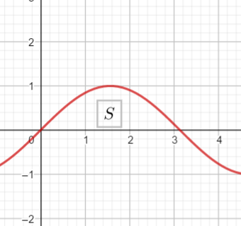
&(1) \text{ If } f(x)\geqslant{0}, \text{ then } \int_{a}^{b}{f(x)dx}=S \quad \text{(Area of the region)}\\
\end{align}\)
\(\begin{align}
&(1) \text{ If } f(x)\geqslant{0}, \text{ then } \int_{a}^{b}{f(x)dx}=S \quad \text{(Area of the region)}\\
\end{align}\)
 \(\begin{align}
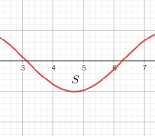
&(2) \text{ If } f(x)\leqslant{0}, \text{ then } \int_{a}^{b}{f(x)dx}=-S\\
\end{align}\)
\(\begin{align}
&(2) \text{ If } f(x)\leqslant{0}, \text{ then } \int_{a}^{b}{f(x)dx}=-S\\
\end{align}\)
 \(\begin{align}
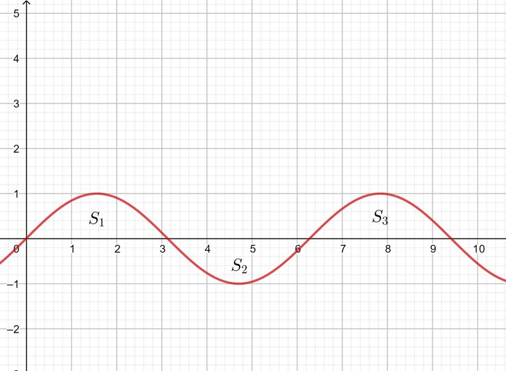
&(3) \text{ If } f(x) \text{ changes sign, then } \int_{a}^{b}{f(x)dx}=S_1+S_3-S_2
\end{align}\)
\(\begin{align}
&(3) \text{ If } f(x) \text{ changes sign, then } \int_{a}^{b}{f(x)dx}=S_1+S_3-S_2
\end{align}\)
II. Properties of Definite Integrals
1. Inequality Properties
\[\begin{align} &(1) \text{ Monotonicity: If } f(x)\leqslant{g(x)} \text{ on } [a,b], \text{ then } \int_a^{b}{f(x)dx}\leqslant{\int_a^{b}{g(x)dx}}\\ \end{align}\] \[\begin{align} &(2) \text{ If } M \text{ and } m \text{ are the maximum and minimum values of } f(x) \text{ on } [a,b] \text{ respectively, then:}\\ &m(b-a)\leqslant{\int_a^{b}{f(x)dx}\leqslant{M(b-a)}}\\ \end{align}\]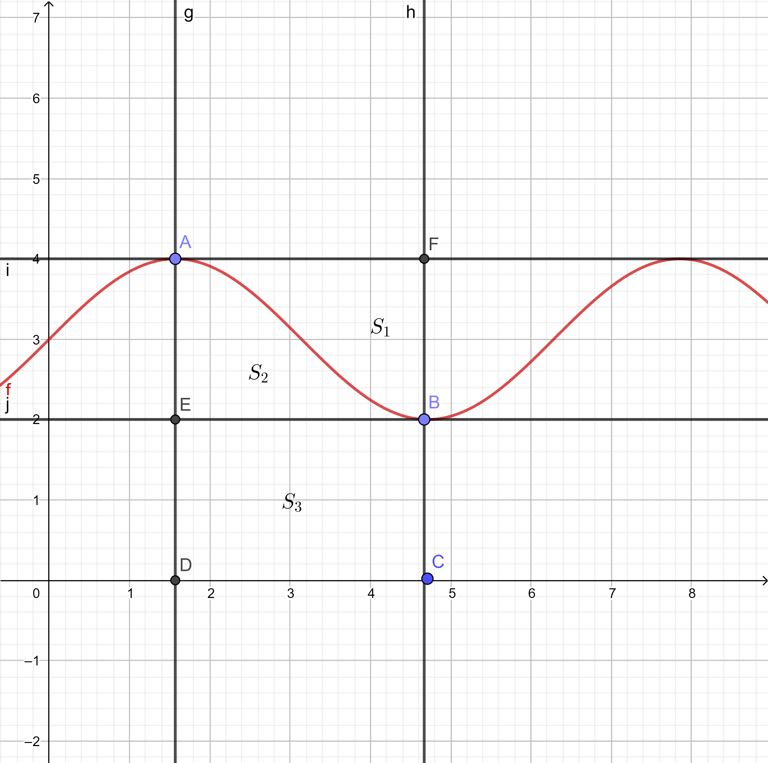 \(\begin{align}
&\text{Proof: } M(b-a)=S_{AFDC}=S_1+S_2+S_3\\
&m(b-a)=S_{EBDC}=S_3\\
&\int_a^{b}{f(x)dx}=S_{ADBC}=S_2+S_3\\
&\because S_3\leqslant{S_2+S_3\leqslant{S_1+S_2+S_3}}\\
&\Leftrightarrow{m(b-a)\leqslant{\int_a^{b}{f(x)dx}\leqslant{M(b-a)}}}\\
\end{align}\)
\(\begin{align}
&\text{Proof: } M(b-a)=S_{AFDC}=S_1+S_2+S_3\\
&m(b-a)=S_{EBDC}=S_3\\
&\int_a^{b}{f(x)dx}=S_{ADBC}=S_2+S_3\\
&\because S_3\leqslant{S_2+S_3\leqslant{S_1+S_2+S_3}}\\
&\Leftrightarrow{m(b-a)\leqslant{\int_a^{b}{f(x)dx}\leqslant{M(b-a)}}}\\
\end{align}\)
2. Mean Value Theorems for Integrals
\[\begin{align} &(1) \text{ If } f(x) \text{ is continuous on } [a,b], \text{ then } \exists \xi \in (a,b) \text{ such that } \int_a^{b}{f(x)dx}=f(\xi)(b-a).\\ &\text{The value } \frac{1}{b-a}{\int_{a}^{b}{f(x)dx}} \text{ is called the average value of } f(x) \text{ on } [a,b].\\ &\text{Note: Let } F'(x)=f(x). \text{ Then } F(b)-F(a)=\int_a^b{f(x)dx}, \text{ and } f(\xi)(b-a)=F'(\xi)(b-a).\\ &(2) \text{ First Mean Value Theorem (Generalized): If } f(x) \text{ and } g(x) \text{ are continuous on } [a,b], \text{ and } g(x) \text{ does not change sign,}\\ &\text{then } \exists \xi \in [a,b] \text{ such that } \int_{a}^{b}{f(x)g(x)dx}=f(\xi)\int_a^b{g(x)dx}.\\ \end{align}\]III. Functions Defined by Integral Upper Limits
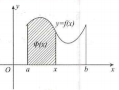 \(\begin{align}
&\text{If } f(x) \text{ is continuous on } [a,b], \text{ then } \Phi(x)=\int_a^x{f(t)dt} \text{ is differentiable on } [a,b], \text{ and:}\\
&\left(\int_a^xf(t)dt\right)'=f(x), \quad \left(\int_a^{x^2}f(t)dt\right)'=f(x^2)\cdot 2x\\
&\text{If } f(x) \text{ is continuous, and } \phi_1(x), \phi_2(x) \text{ are differentiable functions, then:}\\
&\left(\int_{\phi_1(x)}^{\phi_2(x)}{f(t)dt}\right)' = f[\phi_2(x)]\cdot\phi_2'(x)-f[\phi_1(x)]\cdot\phi_1'(x)\\
&\text{Explanation: This follows from } \left(\int_{\phi_1(x)}^0{f(t)dt}+\int_0^{\phi_2(x)}{f(t)dt}\right)'\\
&\text{Let } f(x) \text{ be continuous on } [-l,l], \text{ then:}\\
&\text{If } f(x) \text{ is an odd function, then } \int_0^xf(t)dt \text{ must be an even function.}\\
&\text{If } f(x) \text{ is an even function, then } \int_0^xf(t)dt \text{ must be an odd function.}\\
\end{align}\)
\(\begin{align}
&\text{If } f(x) \text{ is continuous on } [a,b], \text{ then } \Phi(x)=\int_a^x{f(t)dt} \text{ is differentiable on } [a,b], \text{ and:}\\
&\left(\int_a^xf(t)dt\right)'=f(x), \quad \left(\int_a^{x^2}f(t)dt\right)'=f(x^2)\cdot 2x\\
&\text{If } f(x) \text{ is continuous, and } \phi_1(x), \phi_2(x) \text{ are differentiable functions, then:}\\
&\left(\int_{\phi_1(x)}^{\phi_2(x)}{f(t)dt}\right)' = f[\phi_2(x)]\cdot\phi_2'(x)-f[\phi_1(x)]\cdot\phi_1'(x)\\
&\text{Explanation: This follows from } \left(\int_{\phi_1(x)}^0{f(t)dt}+\int_0^{\phi_2(x)}{f(t)dt}\right)'\\
&\text{Let } f(x) \text{ be continuous on } [-l,l], \text{ then:}\\
&\text{If } f(x) \text{ is an odd function, then } \int_0^xf(t)dt \text{ must be an even function.}\\
&\text{If } f(x) \text{ is an even function, then } \int_0^xf(t)dt \text{ must be an odd function.}\\
\end{align}\)
IV. Evaluation of Definite Integrals
1. Newton-Leibniz Formula
\[\int_a^bf(x)dx=F(x)\bigg|_a^b=F(b)-F(a)\]2. Integration by Substitution
\[\int_a^bf(x)dx=\int_\alpha^\beta{f(\Phi(t))\Phi'(t)dt} \quad (\text{where } a=\Phi(\alpha), b=\Phi(\beta))\]3. Integration by Parts
\[\int_a^budv=uv\bigg|_a^b-\int_a^bvdu\]4. Symmetry and Periodicity
\[\begin{align} &(1) \text{ Let } f(x) \text{ be continuous on } [-a,a] \, (a>0), \text{ then:}\\ &\int_{-a}^{a}f(x)dx=\begin{cases}0,&f(x) \text{ is an odd function}\\2\int_0^af(x)dx,&f(x) \text{ is an even function}\end{cases}\\ &(2) \text{ Let } f(x) \text{ be a continuous periodic function with period } T, \text{ then for any } a:\\ &\int_a^{a+T}f(x)dx=\int_0^T{f(x)dx}\\ \end{align}\]5. Useful Formulas
\[\begin{align} &(1) \text{ Wallis' Formulas (or Improper/Definite Symmetric Reduction formula):}\\ &\int_0^{\frac{\pi}{2}}{\sin^nxdx}=\int_0^{\frac{\pi}{2}}\cos^n xdx=\begin{cases}\frac{n-1}{n}\cdot\frac{n-3}{n-2}\cdot\dots\cdot\frac{1}{2}\cdot\frac{\pi}{2},&n \text{ is even}\\\frac{n-1}{n}\cdot\frac{n-3}{n-2}\cdot\dots\cdot\frac{2}{3},&n \text{ is an odd number greater than 1}\end{cases}\\ &(2) \int_0^{\pi}xf(\sin x)dx=\frac{\pi}{2}\int_0^{\pi}f(\sin x)dx \quad (\text{where } f(x) \text{ is a continuous function})\\ \end{align}\]6. Classic Examples:
Example 1:
\[\begin{align} &\text{Evaluate } \lim_{n\rightarrow \infty}{\left(\frac{1}{n+1}+\frac{1}{n+2}+\dots+\frac{1}{n+n}\right)}\\ &\text{Method 1: Squeeze Theorem + Basic Inequalities}\\ &\text{Using } \frac{1}{1+x}<\ln(x+1)<x \text{ for } x>0:\\ &\text{Let } x=\frac{1}{n}:\\ &\frac{1}{n+1}=\frac{\frac{1}{n}}{\frac{1}{n}+1}<\ln\left(\frac{1}{n}+1\right)=\ln(n+1)-\ln(n)<\frac{1}{n}\\ &\text{Similarly: } \frac{1}{n+2}<\ln(n+2)-\ln(n+1)<\frac{1}{n+1}\\ &\dots\\ &\frac{1}{n+n}<\ln(n+n)-\ln(n+n-1)<\frac{1}{n+n-1}\\ &\text{Summing these up gives: } \frac{1}{n+1}+\frac{1}{n+2}+\dots+\frac{1}{n+n}<\ln(2n)-\ln(n)=\ln 2\\ &\text{Method 2: Riemann Sum (Definite Integral Definition)}\\ &\text{In the expression } \lim_{n\rightarrow \infty}{\left(\frac{1}{n+1}+\frac{1}{n+2}+\dots+\frac{1}{n+n}\right)}:\\ &n \text{ is the base part, while } 1, 2, \dots, n \text{ are the variable parts.}\\ &\frac{\text{variable part}}{\text{base part}} \xrightarrow{n \rightarrow{\infty}} \begin{cases}0, \text{ different order (Squeeze Theorem required)}\\A\neq 0, \text{ same order (Definite Integral applies)}\end{cases}\\ &\lim_{\lambda \rightarrow 0}{\sum_{i=1}^{n}{f(\xi_i)\Delta x_i}}=\lim_{n\rightarrow \infty}\frac{1}{n}\sum_{i=1}^{n}f\left(\frac{i}{n}\right) = \int_0^1\frac{1}{1+x}dx=\ln(1+x)\bigg|_{0}^{1}=\ln2\\ \end{align}\]Example 2
\[\begin{align} &\text{Let } f(x)=\int_0^{x}{\frac{\sin t}{\pi-t}dt}, \text{ compute } \int_0^{\pi}f(x)dx. \quad \text{(Correction of typo in prompt's upper bound variables)}\\ &\text{Method 1: Integration by Parts + Substitution}\\ &\text{Integral} = xf(x)\bigg|_0^{\pi}-\int_0^{\pi}{x f'(x)dx}\\ &=\pi{\int_0^{\pi}{\frac{\sin{t}}{\pi-t}dt}-\int_0^{\pi}{\frac{x\sin x}{\pi-x}}dx}\\ &=\int_0^{\pi}{\frac{(\pi-x)\sin x}{\pi-x}dx}=\int_0^{\pi}\sin x dx=2\\ &\text{Method 2:}\\ &\text{Integral} = \int_0^\pi{f(x)d(x-{\pi})}=(x-\pi)f(x)\bigg|_0^{\pi}-\int_0^{\pi}{\frac{(x-\pi)\sin x}{\pi-x}dx}=0 - \int_0^\pi (-\sin x)dx = 2\\ &\text{Method 3: Double Integral converted to Iterated Integral}\\ &\text{Integral} = \int_0^{\pi}{\int_0^{x}\frac{\sin t}{\pi-t}dt}dx\\ \end{align}\]Example 3

 \(\begin{align}
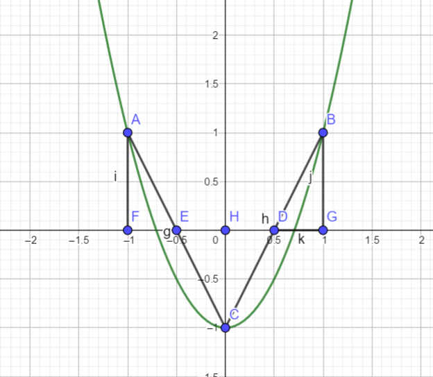
&\text{Method 1: Construct an auxiliary function}\\
&\text{From the problem description, } f(1)=f(-1)=1, f(0)=-1 \Rightarrow f(x) \text{ is an even function, with its minimum value at } -1.\\
&\text{We can construct an auxiliary function that satisfies the conditions: } f(x)=2x^2-1.\\
&\text{Method 2: Direct determination based on functional properties.}
\end{align}\)
\(\begin{align}
&\text{Method 1: Construct an auxiliary function}\\
&\text{From the problem description, } f(1)=f(-1)=1, f(0)=-1 \Rightarrow f(x) \text{ is an even function, with its minimum value at } -1.\\
&\text{We can construct an auxiliary function that satisfies the conditions: } f(x)=2x^2-1.\\
&\text{Method 2: Direct determination based on functional properties.}
\end{align}\)
Example 4
AZZK.jpg)
Improper Integrals
I. Improper Integrals over Infinite Intervals
\[\begin{align} &(1) \int_a^{+\infty}{f(x)}dx=\lim_{t\rightarrow +\infty}{\int_{a}^{t}f(x)dx}\\ &(2) \int_{-\infty}^{b}{f(x)}dx=\lim_{t\rightarrow -\infty}{\int_{t}^{b}f(x)dx}\\ &(3) \text{ If both } \int_{-\infty}^{0}{f(x)}dx \text{ and } {\int_{0}^{+\infty}f(x)dx} \text{ converge, then } {\int_{-\infty}^{+\infty}f(x)dx} \text{ converges, and:}\\ &{\int_{-\infty}^{+\infty}f(x)dx}=\int_{-\infty}^{0}{f(x)}dx+{\int_{0}^{+\infty}f(x)dx}\\ &\text{If at least one of them diverges, the entire integral diverges.}\\ &\text{Common Conclusion: } \int_a^{+\infty}{\frac{1}{x^p}dx} \begin{cases}\text{converges}, &p>1\\\text{diverges}, &p\leq1\end{cases} \quad (a>0)\\ \end{align}\]II. Improper Integrals of Unbounded Functions (Inproper Integrals with Vertical Asymptotes)
\[\begin{align} &\text{If a function } f(x) \text{ is unbounded in any neighborhood of point } a, \text{ then } a \text{ is called a singular point (or vertical asymptote).}\\ &\text{An improper integral of an unbounded function is also called a singular integral.}\\ &(1) \text{ Let } f(x) \text{ be continuous on } (a,b], \text{ where } a \text{ is a singular point. If the limit } \lim_{t\rightarrow a^+}{\int_{t}^{b}{f(x)dx}} \text{ exists,}\\ &\text{then this limit is defined as the improper integral of } f(x) \text{ on } [a,b], \text{ denoted as } \int_{a}^{b}f(x)dx = \lim_{t\rightarrow a^+}{\int_{t}^{b}{f(x)dx}}.\\ &\text{In this case, the improper integral converges; if the limit does not exist, it diverges.}\\ &(2) \text{ If } f(x) \text{ is continuous on } [a,b) \text{ and } b \text{ is a singular point, the improper integral is defined as: } \int_a^bf(x)dx=\lim_{t\rightarrow b^-}{\int_a^tf(x)dx}\\ &(3) \text{ If } f(x) \text{ is continuous on } [a,b] \text{ except at point } c \, (a<c<b), \text{ which is a singular point, and if both}\\ &\int_a^c{f(x)dx} \text{ and } \int_c^b{f(x)dx} \text{ converge, then } \int_a^b{f(x)dx} \text{ converges, and:}\\ &\int_a^b{f(x)dx}=\int_a^c{f(x)dx}+\int_c^b{f(x)dx}\\ &\text{If either diverges, then } \int_a^b{f(x)dx} \text{ diverges.}\\ &\text{Common Conclusions:}\\ &\int_a^b{\frac{1}{(x-a)^p}dx} \begin{cases}\text{converges}, &p<1\\\text{diverges}, &p\geq 1\end{cases}\\ &\int_a^b{\frac{1}{(b-x)^p}dx} \begin{cases}\text{converges}, &p<1\\\text{diverges}, &p\geq 1\end{cases}\\ \end{align}\]III. Examples
Example 1
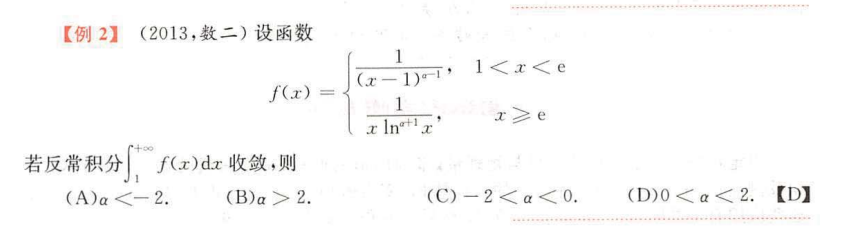 \(\begin{align}
&\int\frac{1}{\ln^{\alpha}x}d(\ln x) \xrightarrow{\ln x=u}\int{\frac{du}{u^{\alpha}}} \dots \text{Comparing with standard forms:}\\
&\text{For convergence at infinity and singular boundaries: } \Rightarrow 0<\alpha<2\\
\end{align}\)
\(\begin{align}
&\int\frac{1}{\ln^{\alpha}x}d(\ln x) \xrightarrow{\ln x=u}\int{\frac{du}{u^{\alpha}}} \dots \text{Comparing with standard forms:}\\
&\text{For convergence at infinity and singular boundaries: } \Rightarrow 0<\alpha<2\\
\end{align}\)
Applications of Definite Integrals
I. Geometric Applications
1. Area of Plane Regions
\[\begin{align} &(1) \text{ If a plane region } D \text{ is bounded by curves } y=f(x), y=g(x) \, (f(x)\geq g(x)), \text{ and lines } x=a, x=b \, (a<b), \text{ the area is:}\\ &S=\int_a^b{[f(x)-g(x)]dx}\\ &(2) \text{ If a plane region is bounded by a polar curve } \rho=\rho(\theta) \text{ and rays } \theta=\alpha, \theta=\beta \, (\alpha<\beta), \text{ the area is:}\\ &S=\frac{1}{2}\int_{\alpha}^{\beta}{\rho^2(\theta)d\theta} \end{align}\]2. Volume of Solids of Revolution
\[\begin{align} &\text{Let a region } D \text{ be bounded by the curve } y=f(x) \, (f(x)\geq 0), \text{ lines } x=a, x=b \, (0\leq a<b), \text{ and the } x\text{-axis:}\\ &(1) \text{ The volume of the solid generated by revolving } D \text{ around the } x\text{-axis for one revolution is: } V_x=\pi\int_a^b{f^2(x)dx}\\ &(2) \text{ The volume of the solid generated by revolving } D \text{ around the } y\text{-axis for one revolution is: } V_y=2\pi\int_a^b{xf(x)dx}\\ &(3) \text{ Generalized Shell Method around any line } y=kx+b \text{ involves the distance } r(x,y): V=2\pi\iint_D r(x,y)d\sigma\\ &\text{Example: Find the volume of the closed region bounded by } y=x \text{ and } y=x^2 \text{ in the first quadrant revolved around lines.}\\ \end{align}\]HIN4FCVUKI$$%5DZB.jpg) \(\begin{align}
&V_x=2\pi\iint_D yd\sigma=2\pi\int_0^1{dx}\int_{x^2}^{x}ydy = \pi \int_0^1 (x^2 - x^4)dx\\
&V_y=2\pi\iint_D xd\sigma=2\pi\int_0^1{dx}\int_{x^2}^{x}xdy = 2\pi \int_0^1 (x^2 - x^3)dx\\
&V_{x=1}=2\pi\iint_D (1-x)d\sigma\\
&V_{y=2}=2\pi\iint_D (2-y)d\sigma\\
\end{align}\)
\(\begin{align}
&V_x=2\pi\iint_D yd\sigma=2\pi\int_0^1{dx}\int_{x^2}^{x}ydy = \pi \int_0^1 (x^2 - x^4)dx\\
&V_y=2\pi\iint_D xd\sigma=2\pi\int_0^1{dx}\int_{x^2}^{x}xdy = 2\pi \int_0^1 (x^2 - x^3)dx\\
&V_{x=1}=2\pi\iint_D (1-x)d\sigma\\
&V_{y=2}=2\pi\iint_D (2-y)d\sigma\\
\end{align}\)
3. Arc Length of a Curve
\[\begin{align} &(1) \text{ Cartesian equation } C: y=y(x), a\leq x\leq b: \quad s=\int_a^b{\sqrt{1+y'^2}dx}\\ &(2) \text{ Parametric equations } C: \begin{cases}x=x(t)\\y=y(t)\end{cases}, \alpha \leq t\leq \beta: \quad s=\int_{\alpha}^{\beta}{\sqrt{x'^2+y'^2}dt}\\ &(3) \text{ Polar equation } C: \rho=\rho(\theta), \alpha \leq \theta\leq \beta: \quad s=\int_{\alpha}^{\beta}{\sqrt{\rho^2+\rho'^2}d\theta}\\ \end{align}\]4. Lateral Surface Area of a Solid of Revolution
\[\begin{align} &\text{The lateral surface area generated by revolving the curve } y=f(x) \, (f(x)\geq 0, a\leq x\leq b) \text{ around the } x\text{-axis is:}\\ &S=2\pi\int_a^b{f(x)\sqrt{1+f'^2(x)}dx}\\ \end{align}\]II. Physical Applications
1. Hydrostatic Pressure
2. Work Done by a Variable Force
3. Gravitational Attraction (Rarely tested)
Example 1

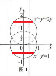
 \(\begin{align}
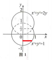
&(2) \text{ Work formula: } W=F\cdot S=G\cdot S=mg\cdot S=\rho g \int V(y) \cdot \text{distance } dy\\
&\text{Upper part work element: } W_1=\rho g \int_{\frac{1}{2}}^{2}(2y-y^2)(2-y)dy\\
&\text{Lower part work element: } W_2=\rho g \int^{\frac{1}{2}}_{-1}(1-y^2)(2-y)dy\\
&\text{Total Work: } W=W_1+W_2\\
\end{align}\)
\(\begin{align}
&(2) \text{ Work formula: } W=F\cdot S=G\cdot S=mg\cdot S=\rho g \int V(y) \cdot \text{distance } dy\\
&\text{Upper part work element: } W_1=\rho g \int_{\frac{1}{2}}^{2}(2y-y^2)(2-y)dy\\
&\text{Lower part work element: } W_2=\rho g \int^{\frac{1}{2}}_{-1}(1-y^2)(2-y)dy\\
&\text{Total Work: } W=W_1+W_2\\
\end{align}\)
Example 2
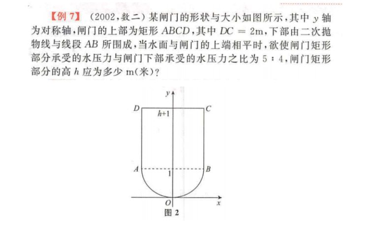 \(\begin{align}
&F_p = \int \rho g \cdot \text{depth} \cdot \text{width} \cdot dy\\
&\text{Divide the gate into upper (rectangular) and lower (parabolic) segments, solving them sequentially:}\\
&P_1=2\rho g \int_1^{h+1}{(h+1-y)\cdot 1} \, dy = \rho g h^2\\
&P_2=2\rho g \int_0^1{(h+1-y)\sqrt{y}dy} = 4\rho g \left(\frac{1}{3}h+\frac{2}{15}\right)\\
&\text{Given } \frac{P_1}{P_2}=\frac{4}{5} \Rightarrow \frac{h^2}{4(\frac{1}{3}h+\frac{2}{15})} = \frac{4}{5} \Rightarrow h=2, \, h=-\frac{4}{15} \text{ (discard negative root). Thus, } h=2.\\
\end{align}\)
\(\begin{align}
&F_p = \int \rho g \cdot \text{depth} \cdot \text{width} \cdot dy\\
&\text{Divide the gate into upper (rectangular) and lower (parabolic) segments, solving them sequentially:}\\
&P_1=2\rho g \int_1^{h+1}{(h+1-y)\cdot 1} \, dy = \rho g h^2\\
&P_2=2\rho g \int_0^1{(h+1-y)\sqrt{y}dy} = 4\rho g \left(\frac{1}{3}h+\frac{2}{15}\right)\\
&\text{Given } \frac{P_1}{P_2}=\frac{4}{5} \Rightarrow \frac{h^2}{4(\frac{1}{3}h+\frac{2}{15})} = \frac{4}{5} \Rightarrow h=2, \, h=-\frac{4}{15} \text{ (discard negative root). Thus, } h=2.\\
\end{align}\)
.jpg)